
Build SLR(1) Parse Table
How to Build SLR(1) Parse Table
The type of LR parsing in JFLAP is SLR(1) Parsing.
S stands for simple LR.
L means the input string is
processed from left to right, as in LL(1) parsing.
R means the
derivation will be a rightmost derivation (the rightmost variable is
replaced at each step).
1 means that one symbol in the input
string is used to help guide the parse.
We will begin by loading the same grammar that we used for building the LL(1) Parse Table. You can enter that grammar or load the file, grammarToLL.jff. After loading the grammar, click on Input and then Build SLR(1) Parse Table. A new rule is automatically added to the grammar, “S'->S”, resulting in a new start variable, “S'”, that does not appear in any right-hand sides. Your window should look like this after entering the SLR(1) Parse mode.
Just like LL(1) Parse, we have to enter the FIRST and FOLLOW sets. If you have not already, read the tutorial on FIRST and FOLLOW sets in the Build LL(1) Parse Table tutorial. After entering proper FIRST and FOLLOW sets, click on Next. You should get a message from JFLAP and your window should look like this :
*NOTE : You can click the Do Step button twice, to make JFLAP automatically fill the FIRST and FOLLOW sets.

We now build a DFA that models the SLR(1) process. Each state will have a label with marked productions called items. The marker is shown as “.”. Those symbols to the left of the marker in an item are already on the parsing stack, and those symbols to the right of the marker still need to be pushed on the parsing stack. All the items for one state are called an item set.
JFLAP now asks you whether you want to define the initial set or not. If you click “Yes”, JFLAP will pop up a small window where you can define the initial set. If you click “No”, then JFLAP will automatically create the initial set for you. Suppose you clicked “Yes”, then you will see a window like this one :

When you click on a production, you will notice that all possible items derivable from that production appear. Since nothing is added to the stack yet, click on the production “S'-> .S”. Since the marker is in front of a variable, “S”, all of the S items with the “.” as the leftmost symbol must be added to the item set. In our grammar, only production “S->.aABb” fits the rule.
*NOTE : You can click on Finish to let JFLAP create the item set for this state. When you are finished, your window should look like this :

You now have your first state “q0” created as shown in the following picture.

*Note : you can make the panel with the state larger by clicking on and moving the horizontal and vertical bars in the window. You may also want to enlarge the window to full screen.
We should add more states and transitions to complete this diagram. First click on the “Goto Set on Symbol” button on the diagram panel, it is the button next to the “arrow” button. From our initial state q0, we know there are only two transitions possible. One is with variable S and the other one is with terminal “a”, since both of these symbols come right after the marker in the item set.
After clicking the “Goto Set on Symbol” button, click on our initial state and drag the mouse and release it at the spot you want to create a new state. Next, JFLAP asks you to enter the symbol for the transition. Let's put variable “S”. When you enter the variable S, you will see the window “Goto on S”. Now click on the production “S'->S.”, since we have moved from our initial state using input “S”, variable “S” is no longer behind the marker. It is now on the left side of the marker. Since there are no variables remaining on the right side of the marker, there is no transition outgoing from the new state. Our completed “Goto on S” should look like this :

We can add another transition from q0 using the terminal “a”. Following the same steps, we will end up with a “Goto on a” window. We add production “S->a.ABb”, since we came to this new state using terminal “a” (this models that “a” is pushed on the parsing stack in the SLR(1) paring process). Now we have to examine the variable “A”, since the marker is in front of it. We add the productions from variable “A”, which start with the marker “.”. There are two productions to add, production “A->.” and “A->.aAc”.
Now after creating these two new states our diagram would look like this :

A state is a final state if one of its items has the marker as the last symbol on the right-side of the production. Since we now know that q1 is one of our final states, we can click the attribute button (“arrow” button), then right click on q1. We can select “final” to make the state q1 final. Try adding the remaining states and their item sets.
After adding all the states (or clicking on Do Step), your final diagram should look like this :

*NOTE : The grammar window's sub-panels are resized to show the diagram.
*NOTE : You can click on the states in the DFA and move them around for a nicer picture.
The DFA is used to build the parse table. Each transition in the DFA results in either a shift entry for a terminal or a goto entry for a variable. Each marked rule with the marker at the right end (found in final states) results in reduce rules.
Now, it's time to fill in entries in the parse table. We can start filling in the parse table from row 0, which corresponds to state q0. From state q0, there are two transitions resulting in two operations. The transition on the “S” relates to “go to” state 1 (q1) and the transition on the “a” relates to “shift” terminal “a” and go to state 2 (q2). Therefore, in the parse table row 0, put s2 (“s” stands for “shift”) in column “a” and put 1 (means just go to state q1) in column S. Now we are done filling the parse table for state q0. Next step is filling in the parse table for q1, which corresponds to row 1. When we reach state q1, we are done parsing since start variable “S” is popped off the stack. So, at state q1, we should accept the string. We fill the entry by typing “acc”, which stands for accepted in column “$”, which implies there are no symbols left to process. After filling in the first two rows of the SLR parse table, your window should look like :

There are two transitions out of state q2. Let's fill in row 2. For transition “a”, we can put “s4” in column “a” in row 2. For transition “A”, we can put the number 3 in column “A” in row 2. Since q2 is a final state, it has at least one reduce rule (a rule with the marker at the right end of the right-side of the rule). The reduce rule is “A->lambda”, shown in JFLAP as “A->.”, and numbered in JFLAP as rule number 3. We can put this reduce rule “r3” in row 2 in columns for all symbols in the FOLLOW(A), which are “b” and “c”. Now we are done with row 2.
*NOTE : There are 4 operations that we use to fill in the parse table : “s” (shift) and “r” (reduce) followed by the destination row number, “acc” for accept, and just a destination row number to indicate transition using variable.
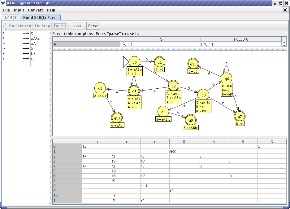
Try filling in the entries for each remaining row. When finished the SLR parse table would look like this :
We have finished the SLR (1) Parse table. Next, click on Parse and in the SLR (1) Parsing window, input “aacbbcb” as the input string. After clicking Start, press Step. Your window should look like this now :

Notice that we have a node with terminal “a” in the tree panel. We achieved the first “a”, so we would remove this “a” from the input remaining. The stack is now filled with “2a0”, meaning that we have reached state 2 from state 0 using transition terminal “a”. You will also notice that the operation that is applied to the input string is highlighted in the parse table, “s2” in the “a” column. Whenever a reduction is applied, both the entry in the parse table and the production that actually performed the reduction will be highlighted. Click Step several times, observing what happens until the string is accepted. The final window should look like one of these :


This concludes our brief tutorial on Building SLR(1) Parse Table. Thanks for reading!